1 Present State of the Particle Method
The particle method is one of simulation methods for solving partial differential equations with spatial discretization. The finite difference method and the finite element method are well known as a spatial discretization method. However, these methods require points and mesh that defines connectivity of points. For example, when solving the solid large deformation from Fig. 1(a) to (b) using the finite element method, the mesh will be distorted and loose accuracy. By contrast, in the particle method, as shown in Fig. 2, it is possible to perform calculations using only information on points. The most important feature of the particle method is that the particles set up virtually in the target body can move freely along with the motion of materials, and therefore each particle can move freely. The particle method is a relatively new computational method that is still growing and developing with improvements. Here we report on present state of the particle method.
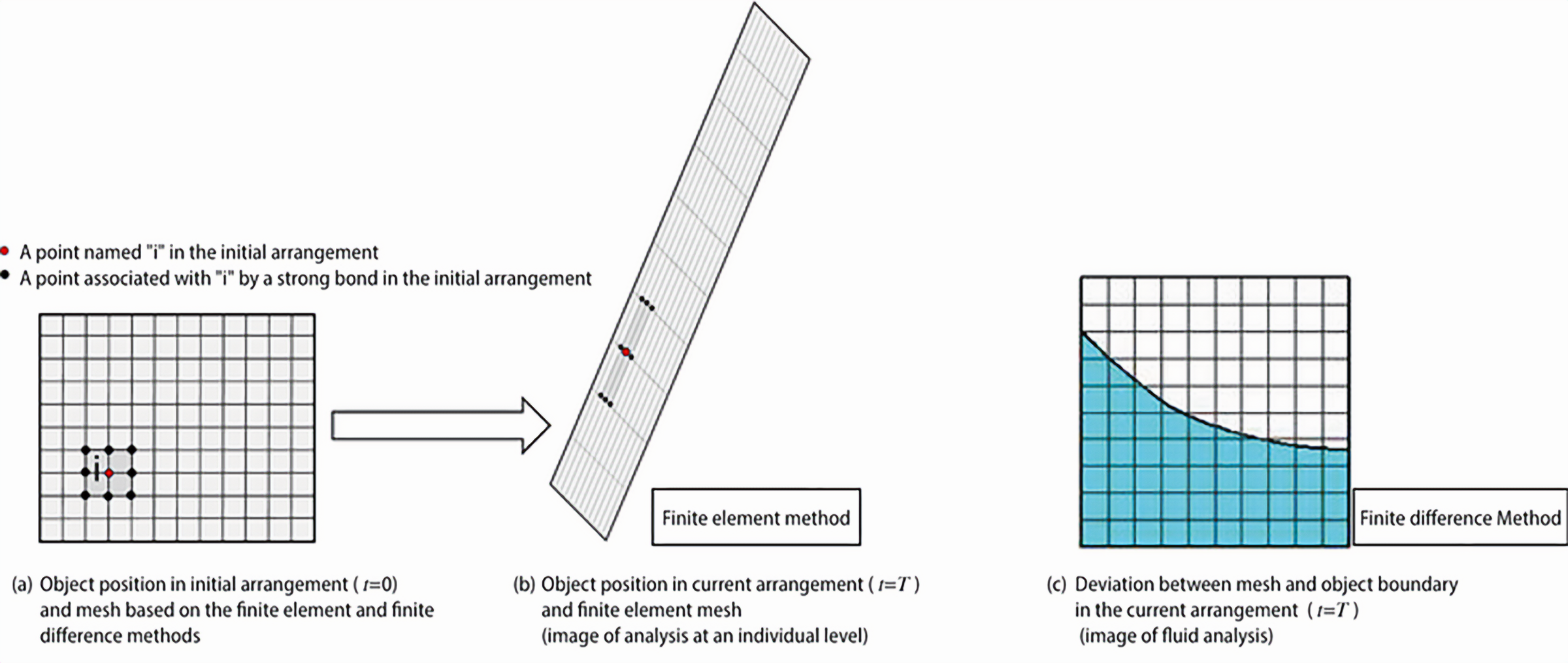
Fig. 1 Images of finite element method and finite difference method
1.1 Historical Development of Particle Method
As explained in the introduction, the finite difference method and the finite element method use both points and meshes. These mesh-based methods, especially in free surface fluid simulation, require split or merge of points in where the surface boundary is significantly deformed, because actual “physical” surface points are different from the initial “numerical” simulation points, as shown in Fig. 1(c). In contrast in the particle simulation, only the points called “particles” can perform these simulations, it serves as an ideal numerical solution tool for large deformation and crack propagation in solid analysis, and for complex surface flows where splashes (repeated water splitting and merging) are generated. Further advantage of the particle method is that it is easier to create analytical models for complex geometries for which meshes are difficult to define since particles can be placed inside the analysis area. The particle method, on the other hand, has only a short development history, and some undergoing developments which should be overcome remain. The major disadvantages are insufficient evaluation of simulation error and complicated boundary treatment without surface boundary points. Recent progress on the particle method, however, has improved both the accuracy of the analysis and the computational stability.
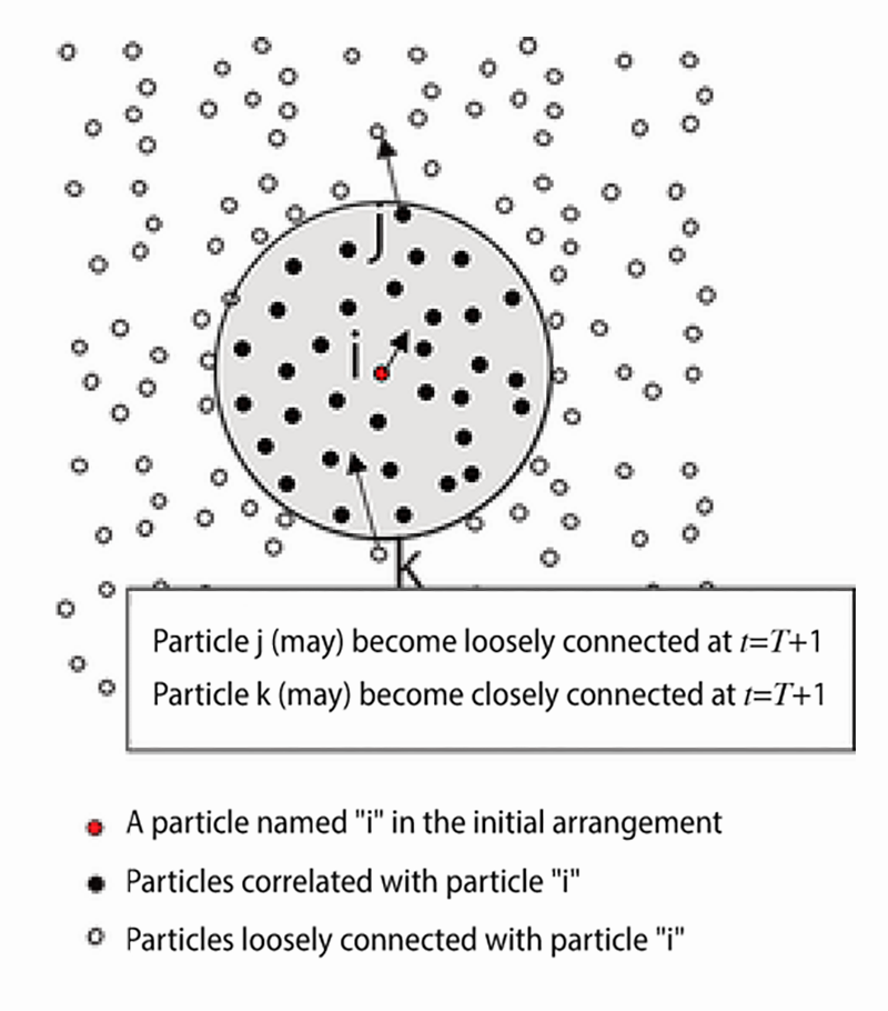
Fig. 2 Image of particle method
This technical column will focus on two representative particle methods, the SPH (Smoothed Particle Hydrodynamics) and the MPS (Moving Particle Semi-implicit method), and explain the similarities between the two methods. After that, we will introduce recently improved features of the particle method in the summary by showing numerical experiments on particle distribution, which is one of the main factors of error. Incidentally, the Distinct/Discrete Element (DEM) method is a particle-based numerical analysis method used to analyze granular materials or multiple rigid blocks. The DEM approximates the interaction force between particles by equivalent springs and dashpots based on empirical rules or physical laws. It is different from the our main topic ‘particle method’ in the sense which the DEM has no partial differential equation as the governing equations.
The SPH was first proposed in 1977 by Lucy [1] and Gingold et al. [2] as a simulation method for astrophysics (e.g., the collision of celestial bodies). The SPH method was developed for compressible fluids [3] in the early 1990s, for incompressible fluids [4] in the late 1990s as a simple extension of compressible fluid solver, and solids after 1990 by Libersky et al. [5] As its basic concept, the SPH method uses a weight function called a “smooth function” to approximate functions. This function is defined for each particle. By directly differentiating this approximate function, we can derive approximate models of the gradient and Laplacian and use them to solve the differential equations approximately.
On the other hand, the MPS method [6,7] proposed by Koshizuka et al. is a particle method similar to the SPH method. However, the derivation process of the gradient and Laplacian and its concept are slightly different. First, the MPS method, unlike the SPH method, started as a method for analyzing incompressible fluids. The MPS is the first method to introduce the semi-implicit scheme with projection method (explicit time integration for velocity and implicit time integration for pressure) into the particle method as a “truly” incompressible flow solver. The MPS method later developed into a fully explicit method by adopting the solution scheme for compressible fluid as in the early SPH method. The approximation of the spatial derivative in the MPS method can be derived as a weighted average of the interactions between particles based on the Taylor expansion of the function (details to be explained in the next issue). By using this approximation, the differential equation can be solved approximately like the SPH method.
As explained above, we see the reversed development in each method: from compressible fluid to incompressible fluid in the SPH method, and from incompressible fluid to compressible fluid in the MPS method in terms of the time integration method and the handling in the incompressibility of fluid. However, now there is no significant difference, including the time integration method. The main difference between the two is spatial discretization, i.e., the approximation method of spatial differentiation, as shown below. The primary difference between the two lies in spatial discretization, or approximation of the spatial derivative. (To be continued to the next column.)
Reference:
[1] L. B. Lucy: A numerical approach to the testing of the fission hypothesis, Astronom. J., Vol. 82, pp. 1013–1024, 1977.
[2] R. A. Gingold and J. J. Monaghan: Smoothed particle hydrodynamics: Theory and application to non-spherical stars, Monthly Not. Roy. Astronom. Soc., Vol. 181(3), pp. 375–389, 1977.
[3] J. J. Monaghan: Simulating free surface flows with SPH, J. Comput. Phys., Vol. 110, pp. 399–406, 1994.
[4] S. J. Cummins and M. Rudman: An SPH projection method, J. Comput. Phys., Vol. 152, pp. 584–607, 1999.
[5] L. D. Libersky and A. Petschek: Smooth particle hydrodynamics with strength of materials, in Advances in the free-Lagrange method including contributions on adaptive gridding and the smooth particle hydrodynamics method, Springer, pp. 248–257, 1991.
[6] S. Koshizuka and Y. Oka: Moving-particle semi-implicit method for fragmentation of incompressible fluid, Nuclear Sci. Eng., Vol. 123, pp. 421-434, 1996.
[7] 越塚誠一:計算力学レクチャーシリーズ5 粒子法, 日本計算工学会編, 丸善, 2005.
TOC
Growing the particle method, and its present state
- Present State of the Particle Method
- Kernel Approximation and Kernel Function Conditions in the SPH Method
(Preparation for Spatial Discretization)
About The Author

Kyushu University, Department of Civil Engineering
Mitsuteru Asai
View Profile
2003, Ph.D. (Tohoku University, Department of Civil Engineering.)
2003-2005, Post-Doctoral Researcher (The Ohio State University)
2005-2007, Assistant Professor (Ritsumeikan University)
2007-, Associate Professor (Kyushu University)