2. In what ways is the particle method different from other methods? | Introduction to the particle method

In the last column, I explained that the particle method can easily solve many difficult problems. Why can the particle method do that? In this column, I would like to explain the reason by comparing the particle method with a conventional mesh-based method. ​

1. Finite Difference Method

The finite difference method (FDM) is a traditional mesh-based method for simulating fluid dynamics. Figure 1 shows a fluid flow, and Fig. 2 shows the conceptual image of the simulated flow by FDM. A simulation domain is discretized by mesh. Calculation points, which are like observation points, are set on certain places in the mesh, such as centers or sides of mesh cells. These calculation points have parameters such as pressure, velocity, fluid density or temperature. The parameters are updated every time step. Basically, calculation mesh is neither moved nor deformed in FDM*1. Therefore, the calculation points also do not move. That is to say, the flow is observed at the same points which are fixed to the space. For example, when we simulate a time change of temperature by FDM, temperatures are evaluated at fixed places. Every time step, temperature of a different fluid element*2 is observed at a place because fluid elements pass through the fixed observation point.

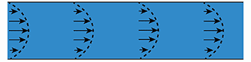
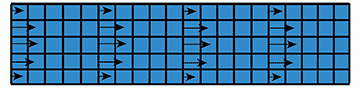
Arrow directions and lengths show their velocity direction and absolute values, respectively. Although each side of a mesh cell has a parameter of velocity, which expresses the absolute value of velocity in vertical direction to the side, only representative arrows are drawn to simplify the figure.

Note 1:

There are some exemptions. For example, the Arbitrary Lagrangian Eulerian (ALE) method moves and deforms the mesh.

Note 2:

An element means substance whose volume is very small. Although elements are not handled directly in FDM, we need to consider the equation of momentum for every fluid element because fluid consists of microscopic elements.

2. Particle method

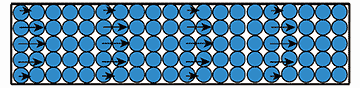
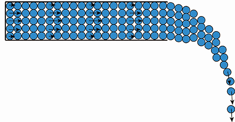
In the particle method, the fluid flow in a pipe shown in Fig. 1 is expressed by particles as shown in Fig.3. A mesh is not necessary. Fluid is expressed by a group of calculation points. Each calculation point is called a particle in the particle method. Each fluid particle expresses small domain of fluid and has parameters for pressure, velocity etc. In contrast to FDM, calculation points in the particle method move in space. The movement velocities of calculation points are the same as their fluid velocities. Because of the movement of calculation points, the particle method is able to be applied to various complex flows such as Fig.4. Movie 1 shows an example of a simulation result obtained by the particle method.

The particle method is simple and easy to implement because we do not need to discretize the advection term of the Navier-Stokes equations. The advection term is called the “convective rate of change” in some books. The advection term is non-linear and complex. The advection term appears when we calculate a substantial derivative*3 by using parameters which are observed at points fixed to the space. In the particle method, we use parameters which follow particles’ movement. Therefore, the advection term does not appear in the particle method.

Let’s compare the particle method with FDM in a case where time change of fluid temperature is calculated. In FDM, the temperature is measured at fixed points. That is to say, the temperature of different fluid particles is calculated every time step. On the other hand, in the particle method the temperature of the same particle is evaluated. Because of this difference, we do not need to calculate the complicated advection term of temperature. In the same manner, the time change of fluid velocity is also easily solved in the particle method without considering the advection term of velocity. That is why the MPS method can easily solve many difficult problems.​

Note 3:

Also called Lagrangian derivative. A time derivative of a physical quantity. The time derivative is evaluated by following a designated substance. That is to say, the evaluation point is moved with the designated substance.